Let’s face it, I am addicted to R, and this is partly (mostly) due to ggplot and Rstudio. If you need an introduction to R, Coursera is a good place to start, as well as swirl. Of course will be small compared to the documentation or the book, but I’ll make it enough to get you started.

Generating data

Thanks to what I learnt on Stack Overflow, I’m making sure that what I’m doing is reproducible - it’s always annoying to see a beautiful example that doesn’t work when you try to reproduce. So we’ll generate data for this (who said mtcars?)

set.seed(123)
dataset<-data.frame(A = sample(x = 1:10, size = 1000, replace = TRUE),
					B = sample(x = LETTERS[1:5], size = 1000, replace = TRUE),
					C = rnorm(n = 1000,mean = 0, sd = 1)
					)
dataset$D<-rnorm(n=1000, mean = dataset$C,sd = 1)

We thus have a dataframe with four columns, A contains integer, B has letters, C and D have numeric values.

plot vs qplot vs ggplot: non-standard evaluation

What is non-standard evaluation? This is the fact that the arguments passed to the aesthetics will not be evaluated, but will be used to call columns. For people used to the plot syntax, it can be disturbing at first, as you should not give vectors as input - we’ll see a workaround to that after. Let’s make this clear with an example of plot, qplot and ggplot:

plot(x= dataset$A, y = dataset$C)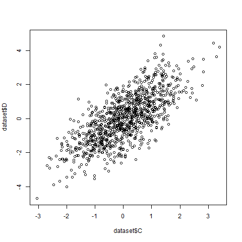

qplot(x= dataset$C, y= dataset$D)

ggplot(data = dataset, aes(x=C,y=D))+geom_point()

Notice:

1. We never explicitely provided the vector in the `ggplot` syntax yet we have the same output as the `qplot`. 
The same syntax is used in `plyr` or `dplyr` (we'll talk about these another time). 
2. The `ggplot` creates an object where characteristics are linked to values, you then have to use to combine this object with a representation `geom_point`
in our case to get a plot! Think of it as an instruction of what you would like to plot.

This is what you should see:

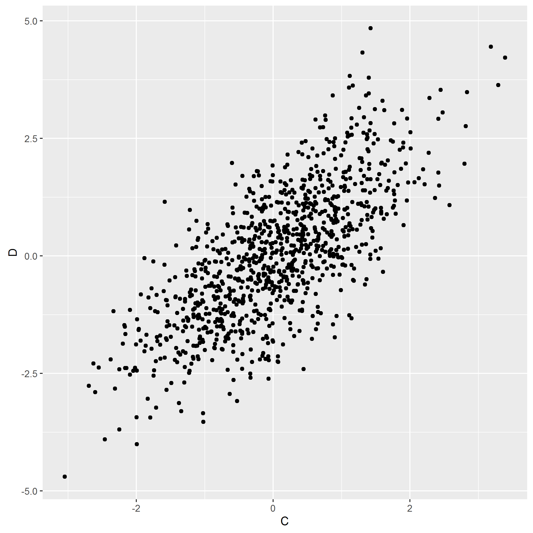
It doesn’t look too good but we’ll make it better.

Editing your plot: basic operations

Changing the theme

By default, the background of ggplot is grey to have a better experience on screens. However, for printing, or by habits, it can be useful to have a black and white theme, or edit the axes. This is feasible with theme(), but some themes are already available with ggplot2, such as theme_bw, theme_classic, or theme_minimal.

ggplot(data = dataset, aes(x=C,y=D))+geom_point()+theme_bw()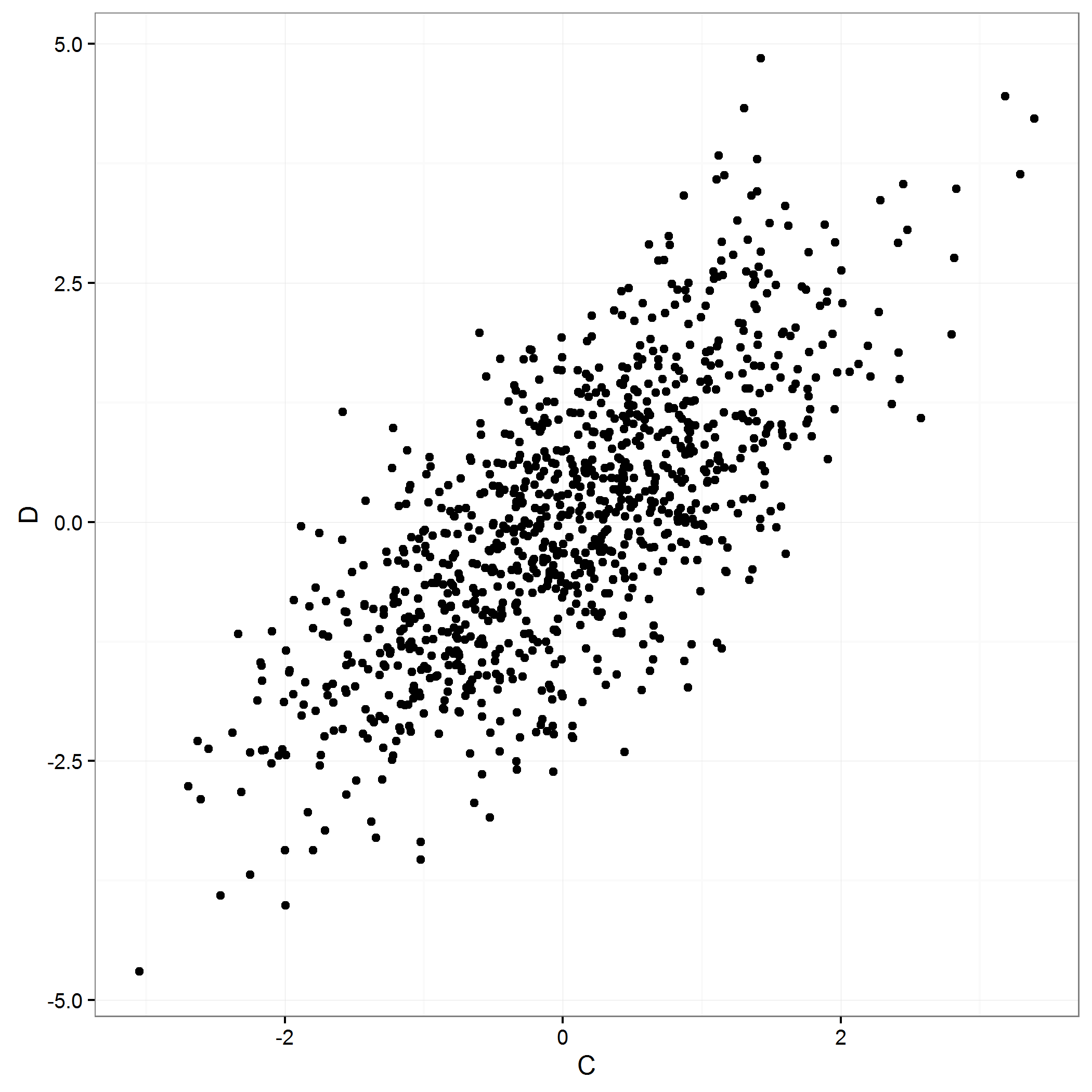

ggplot(data = dataset, aes(x=C,y=D))+geom_point()+theme_classic()

ggplot(data = dataset, aes(x=C,y=D))+geom_point()+theme_minimal()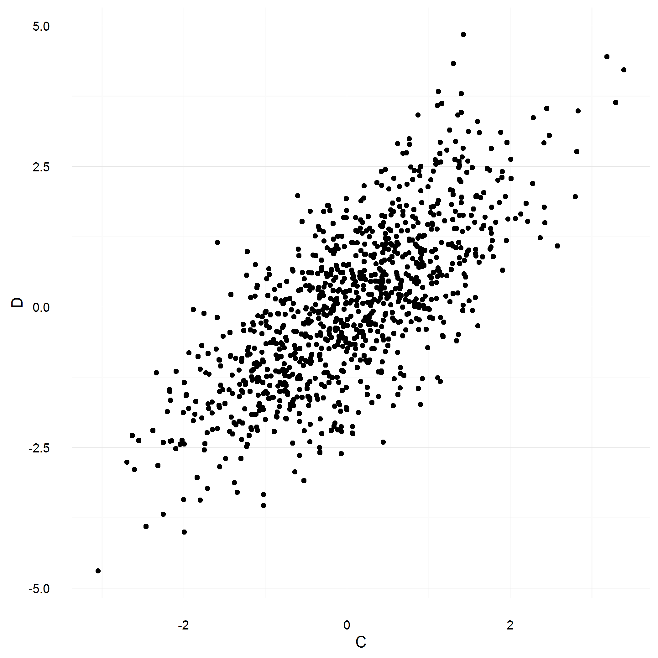

Often, where labels on the axes are quite large, it can be useful to turn them. This is also an operation handled in theme. We’ll keep the black & white theme, and add a 45° shift to the x axis and make it bigger:

ggplot(data = dataset, aes(x=C,y=D))+geom_point()+theme_bw()+
theme(axis.text.x = element_text(angle = 45,size = 16))+
  xlab("X axis")+ylab("Y axis")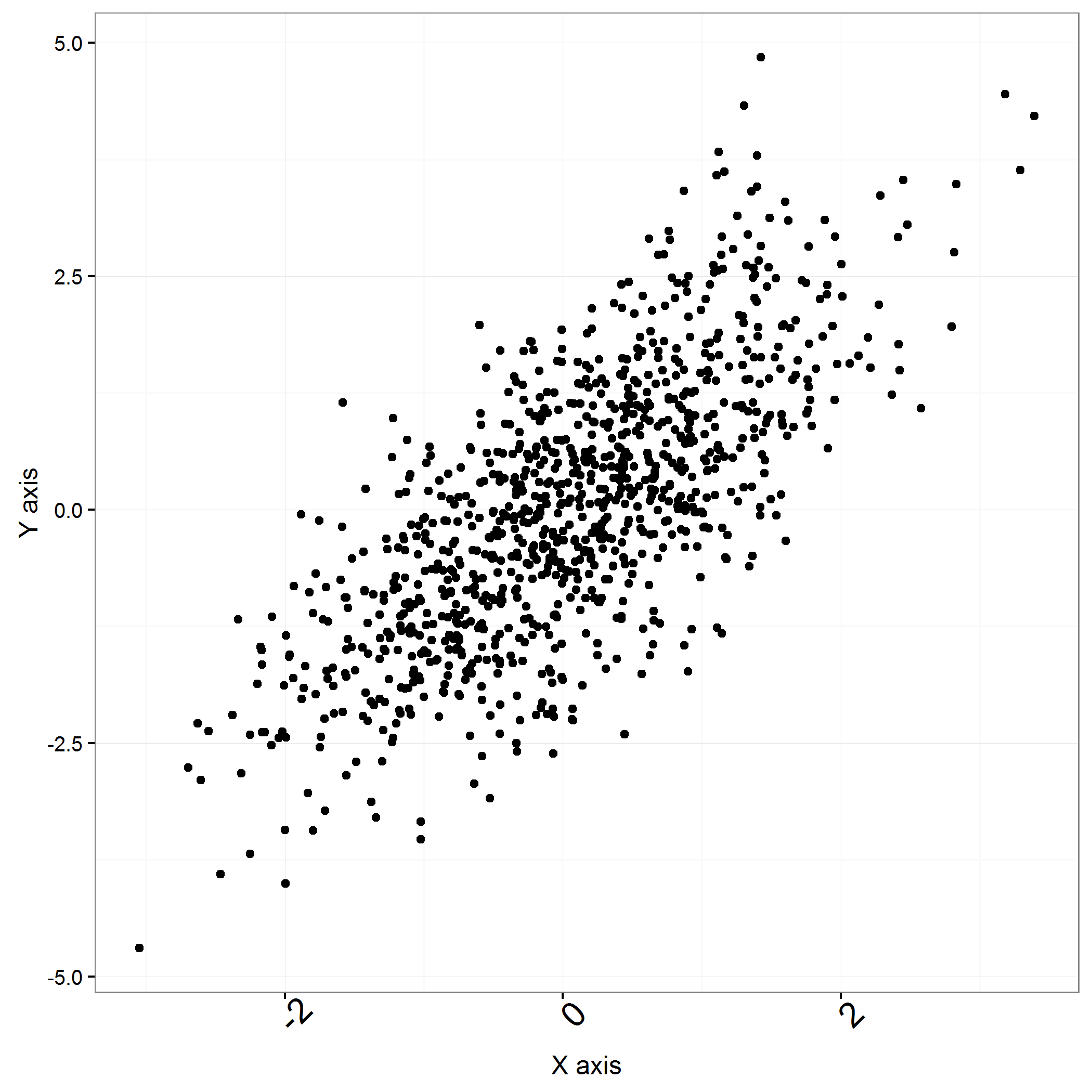

Notice how you can also change the labels of the axes with xlab and ylab. You don’t remember if it is x.ticks.axis or x.axis.ticks to change the ticks in your theme? Don’t worry, everything is listed here (It is axis.ticks.x )

Adding color and editing legend

Now that we have a theme, we will color the points based on values from column A.

ggplot(data = dataset, aes(x=C,y=D,color = A))+geom_point()+theme_bw()

We have a gradient of colors, but our data is integer? ggplot assumes that numerical data are continuous, so the best way to represent these is a gradient. To change that, you need to make this data a factor or a character. Otherwise you will get an error message:

Error: Continuous value supplied to discrete scale

dataset$A<-as.character(dataset$A)
ggplot(data = dataset, aes(x=C,y=D,color = A))+geom_point()+theme_bw()+
			scale_color_discrete("This is \n a legend")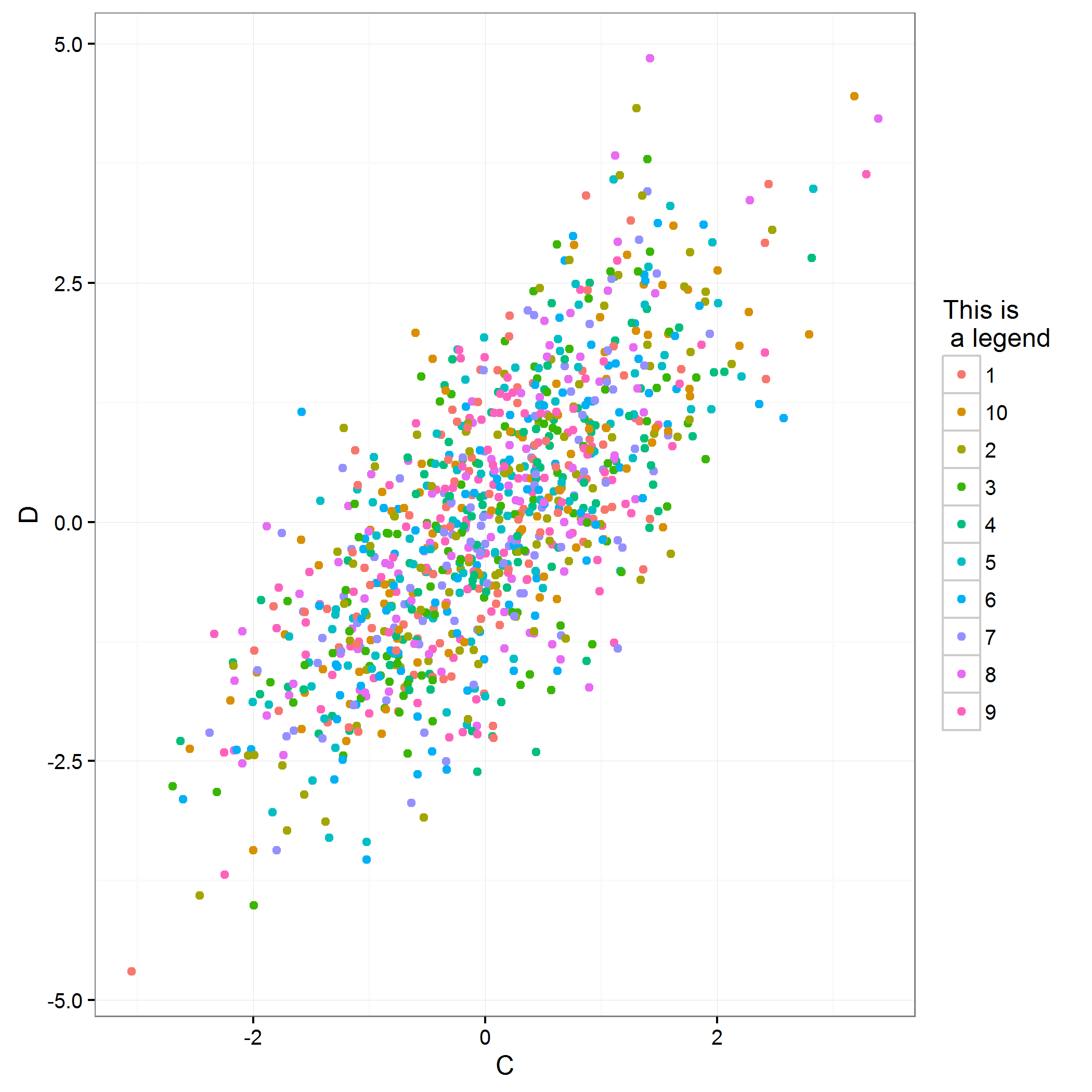

I also provided the name of the legend for colors in the scale_color_discrete, but this legend is ordered in alphabetical order… It would be better in numerical order:

dataset$A<-factor(dataset$A,levels  = 
				unique(dataset$A)[order(as.numeric(unique(dataset$A)))])
ggplot(data = dataset, aes(x=C,y=D,color = A))+geom_point()+theme_bw()+
			scale_color_discrete("This is \n a legend")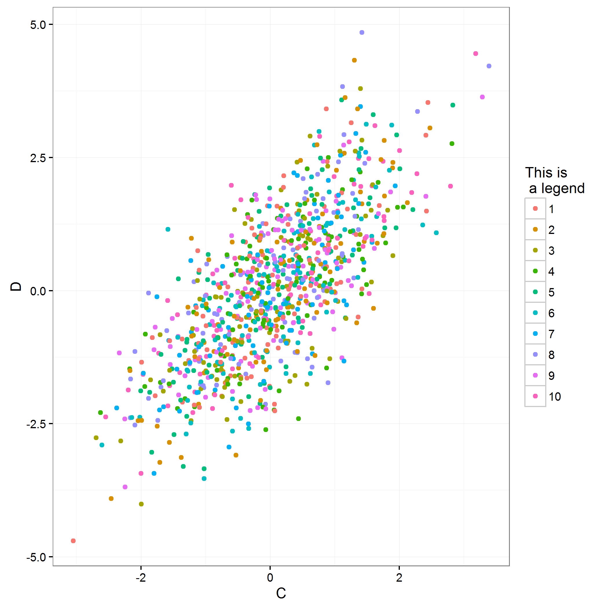

We’ll also add shapes to this plot:

ggplot(data = dataset, aes(x=C,y=D,color = A,shape = B))+geom_point()+theme_bw()+
			scale_color_discrete("This is \n a legend")+scale_shape_discrete("Shape legend")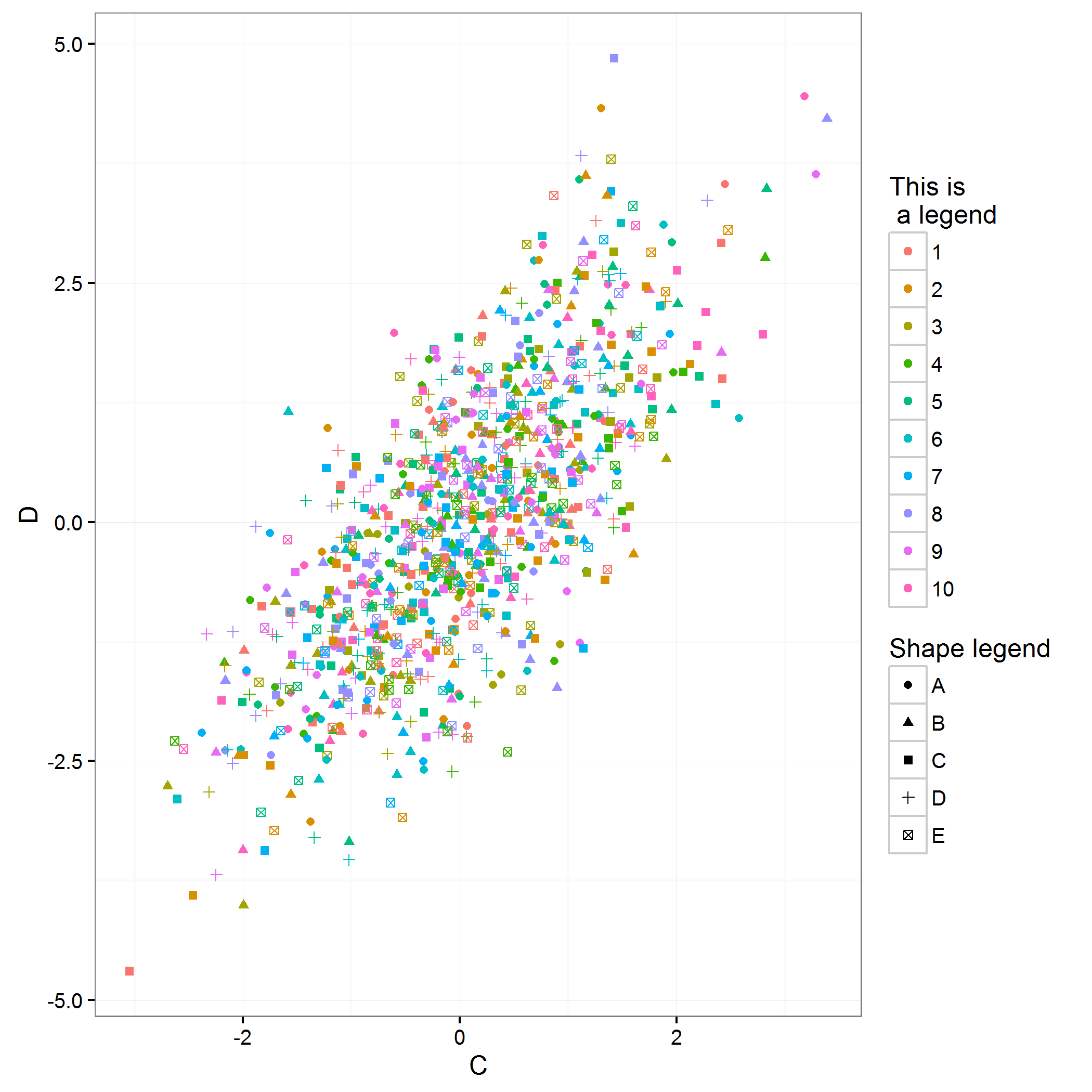

Adding lines

What happens if we try to connect the previous points?

ggplot(data = dataset, aes(x=C,y=D,color = A))+geom_line()+theme_bw()+
			scale_color_discrete("This is \n a legend")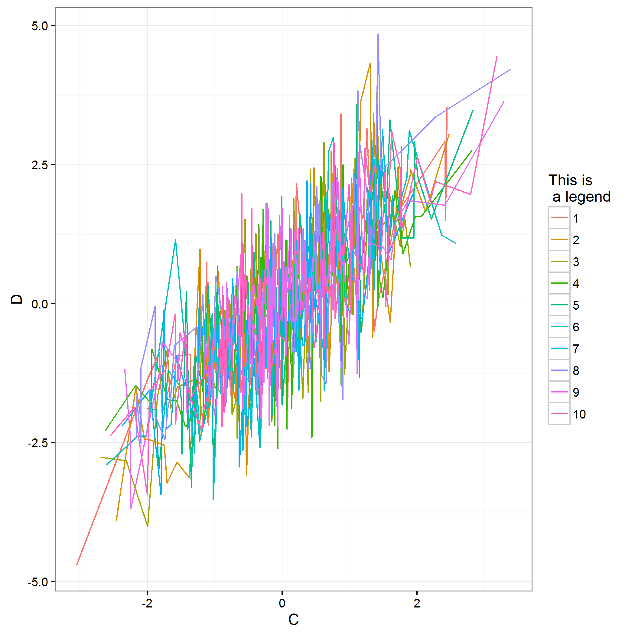

Let’s make it a bit more transparent so that we can see better:

ggplot(data = dataset, aes(x=C,y=D,color = A))+geom_line(alpha = I(0.5))+theme_bw()+
			scale_color_discrete("This is \n a legend")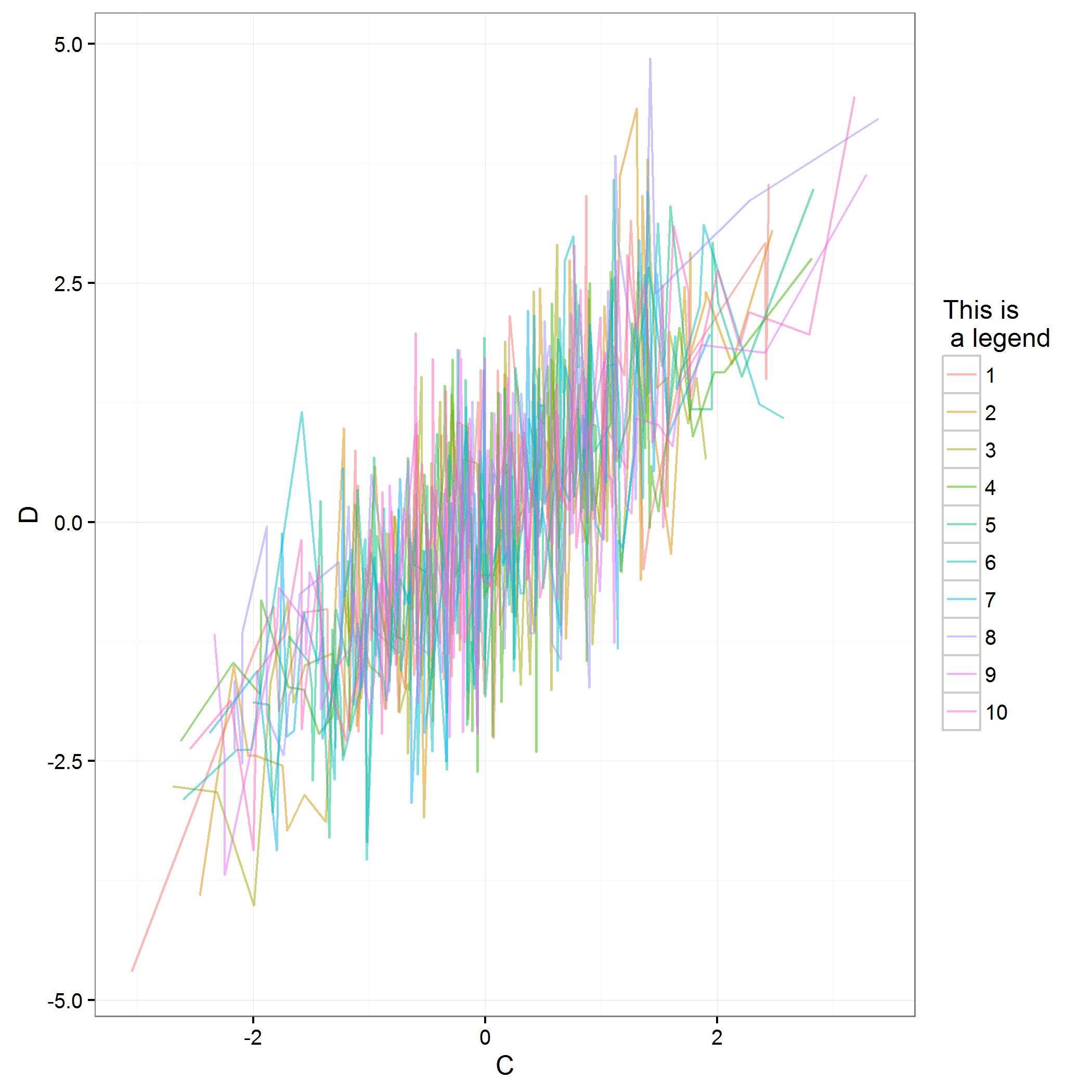

The I function tells ggplot that 0.5 is a numeric value of transparency, and not a value to group different lines. You can now see that each color has its own line! This is because ggplot has grouped the points by values of the color, shape, etc. It is useful to remember this when you want to have a single line with multiple colors.

Adding a trend

Now we know how to make a line, but we’d like a trend for all points and one trend for each color. We’ll try using geom_smooth:

ggplot(data = dataset, aes(x=C,y=D,color = A))+geom_smooth(alpha = I(0.3))+geom_point()+theme_bw()+
  scale_color_discrete("This is \n a legend")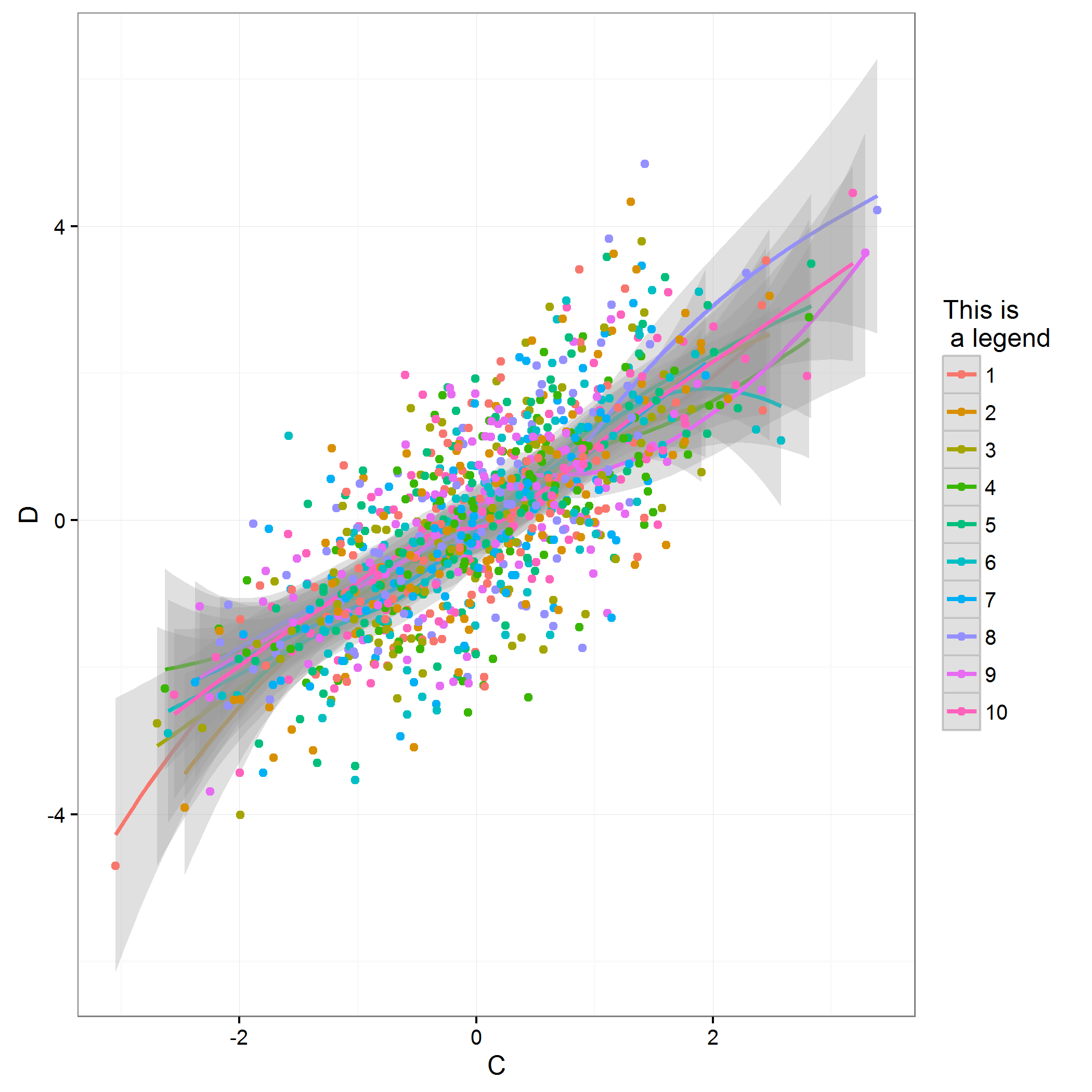

Not very useful to have a trend for each class, is it? Remember, we have grouped everything because of the color in ggplot, so if I remove it, and only use it as an argument in geom_point what happens?

ggplot(data = dataset, aes(x=C,y=D))+geom_smooth(alpha = I(0.3))+geom_point(aes(color = A))+theme_bw()+
  scale_color_discrete("This is \n a legend")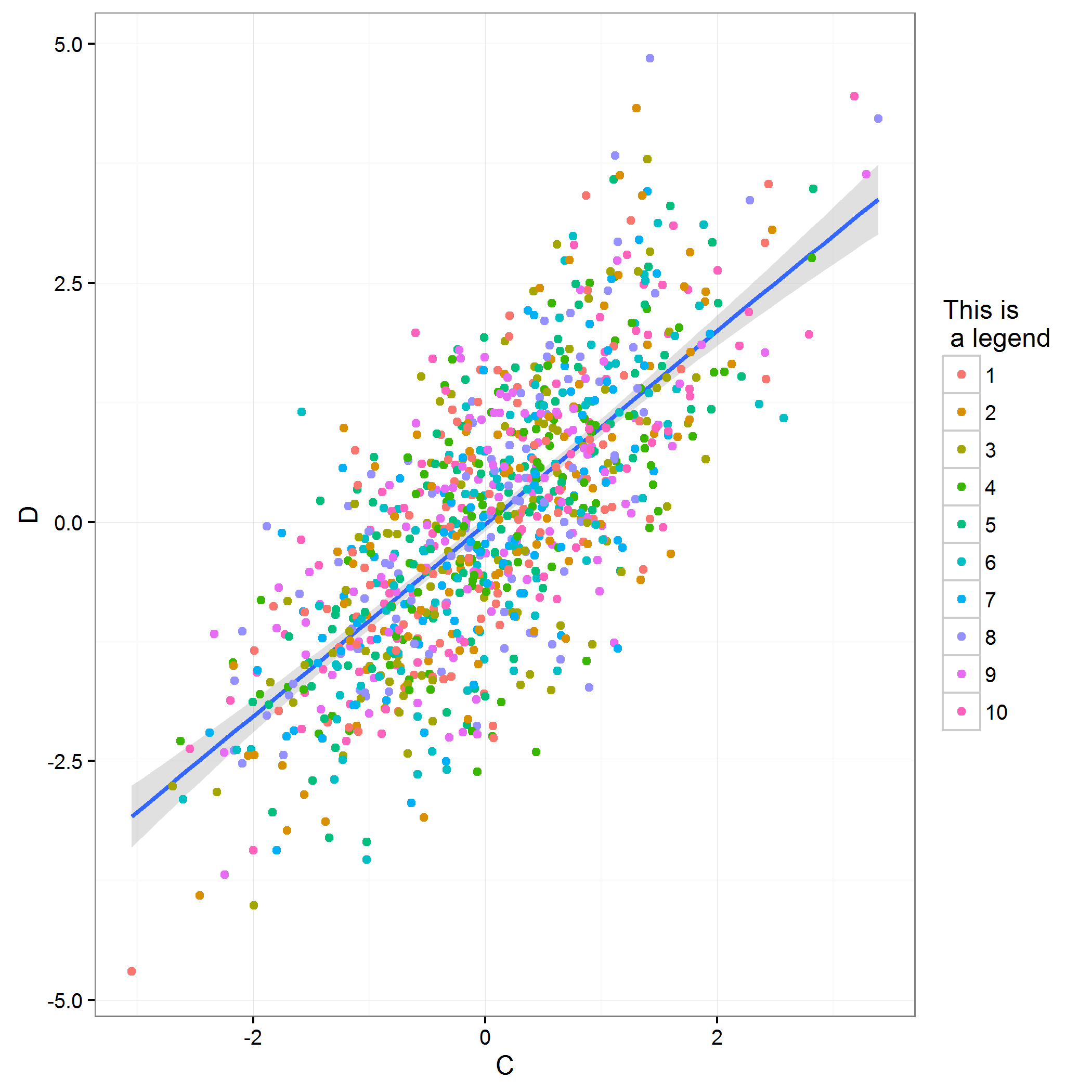

The trend has been calculated on the whole dataset, and we still have our points shown with different colors!

Showing density

We have shown the trend of points, but sometimes it can be more useful to show a density of points, either one or two-dimensional. Here we will show for 2D density, but the same works with geom_density. We also increase the transparency of points in our plot:

ggplot(data = dataset, aes(x=C,y=D))+geom_density_2d()+geom_point(aes(color = A),alpha = I(0.3))+theme_bw()+
  scale_color_discrete("This is \n a legend")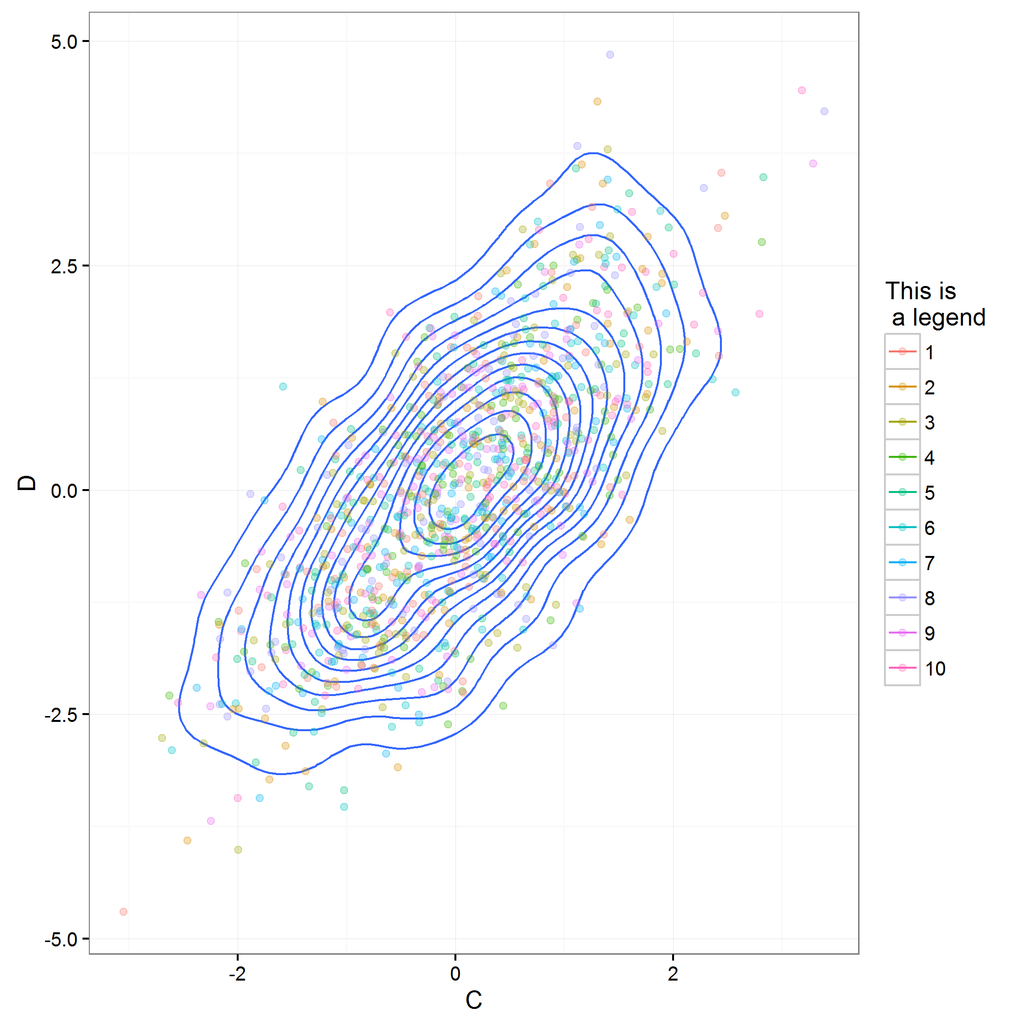

You now know a lot in making plots with ggplot2. One last useful thing is to apply what we have seen with histograms.

Making an histogram

An histogram shows the number of values that fall into a bin, for example in the sequence {0,1,5,7,2,10}, 3 values fall in [0;2].

We are going to make an histogram of our data with 50 bins:

ggplot(data = dataset, aes(x=C))+geom_histogram(bins = 50)+theme_bw()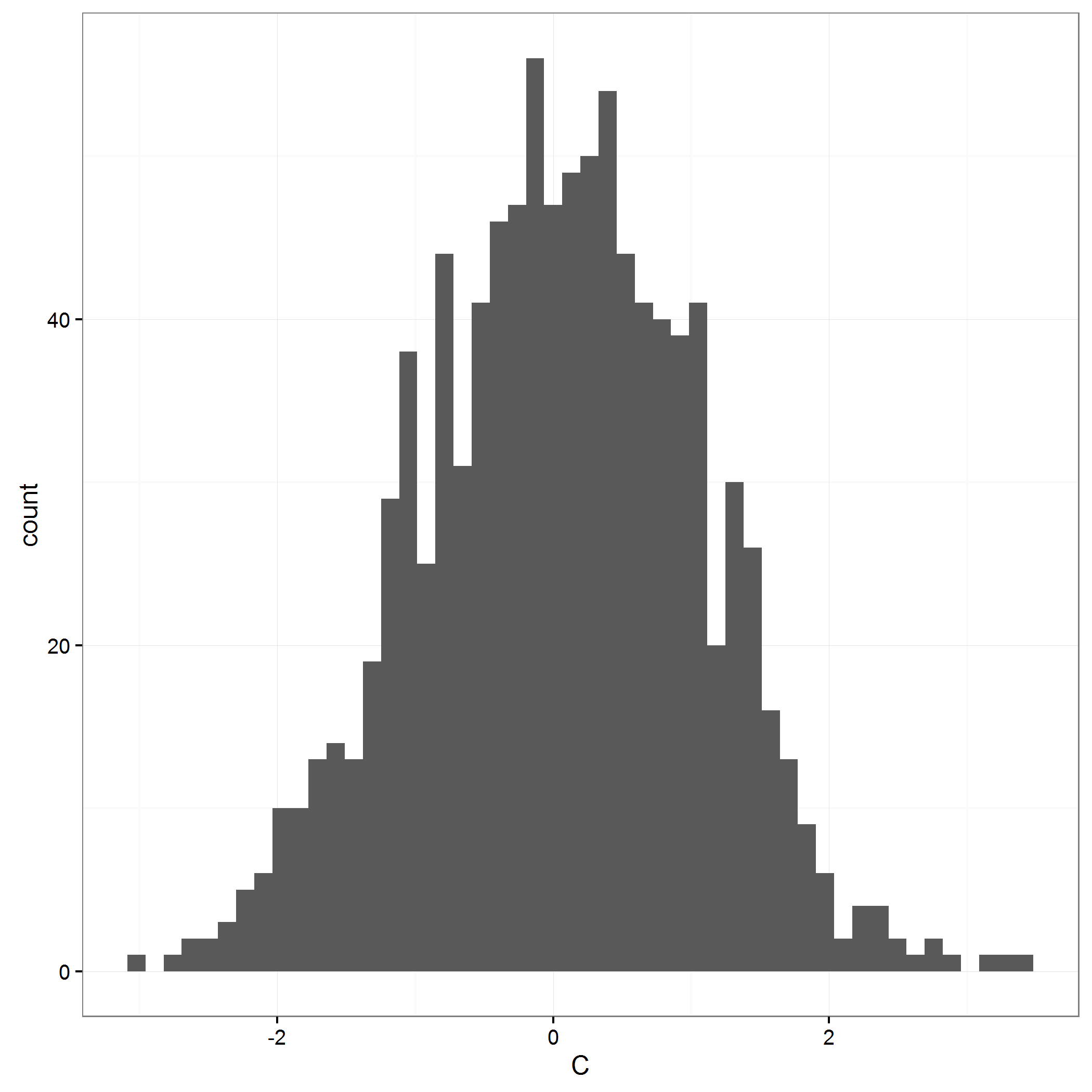

Editing the histogram

How do we add color to this plot? With with the color argument again?

ggplot(data = dataset, aes(x=C,color = B))+geom_histogram(bins = 50)+theme_bw()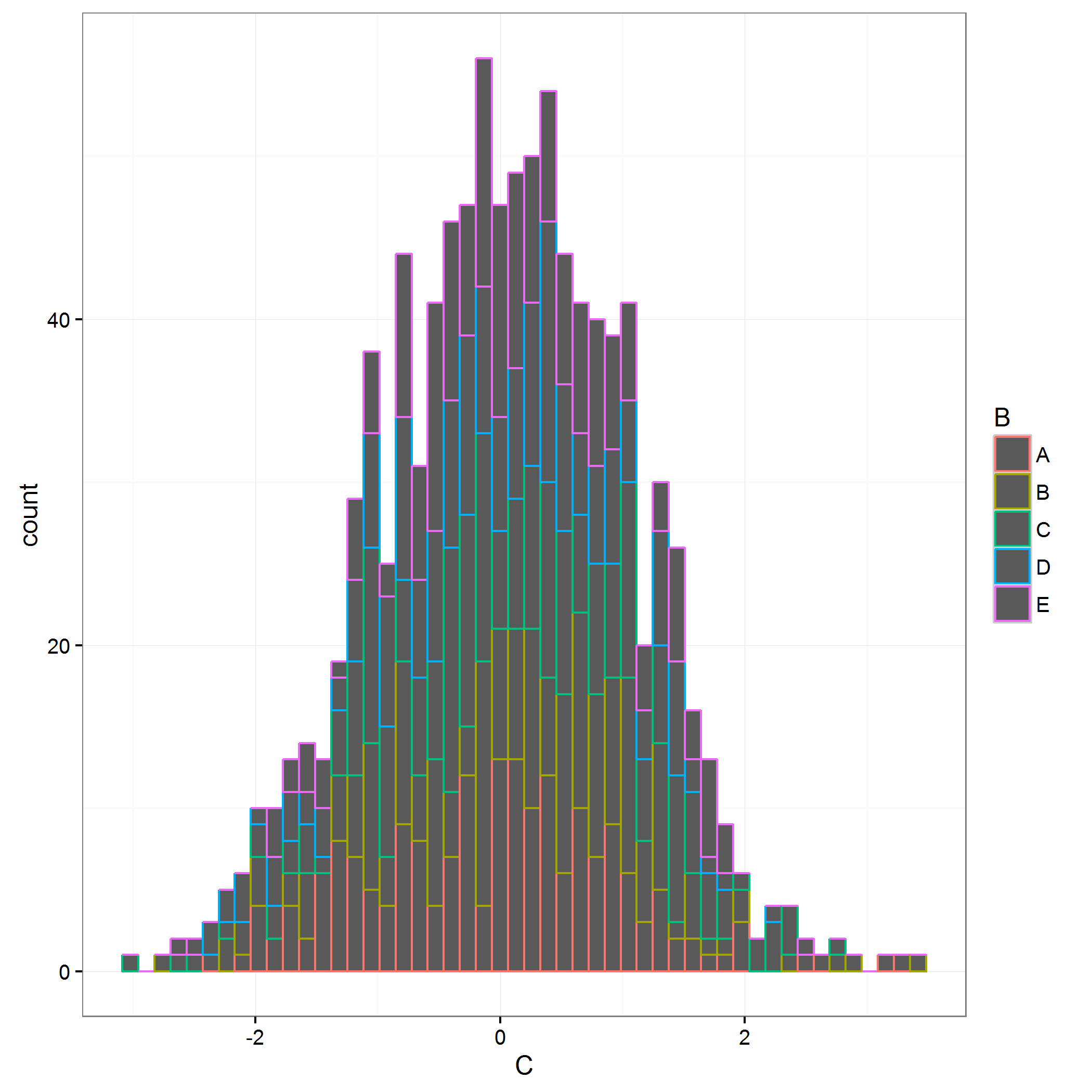

As you can see, only the edge of the bars have been colored. This is because areas have a fill argument.

ggplot(data = dataset, aes(x=C,fill = B))+geom_histogram(bins = 50)+theme_bw()+
  scale_fill_discrete("This is \n a fill ")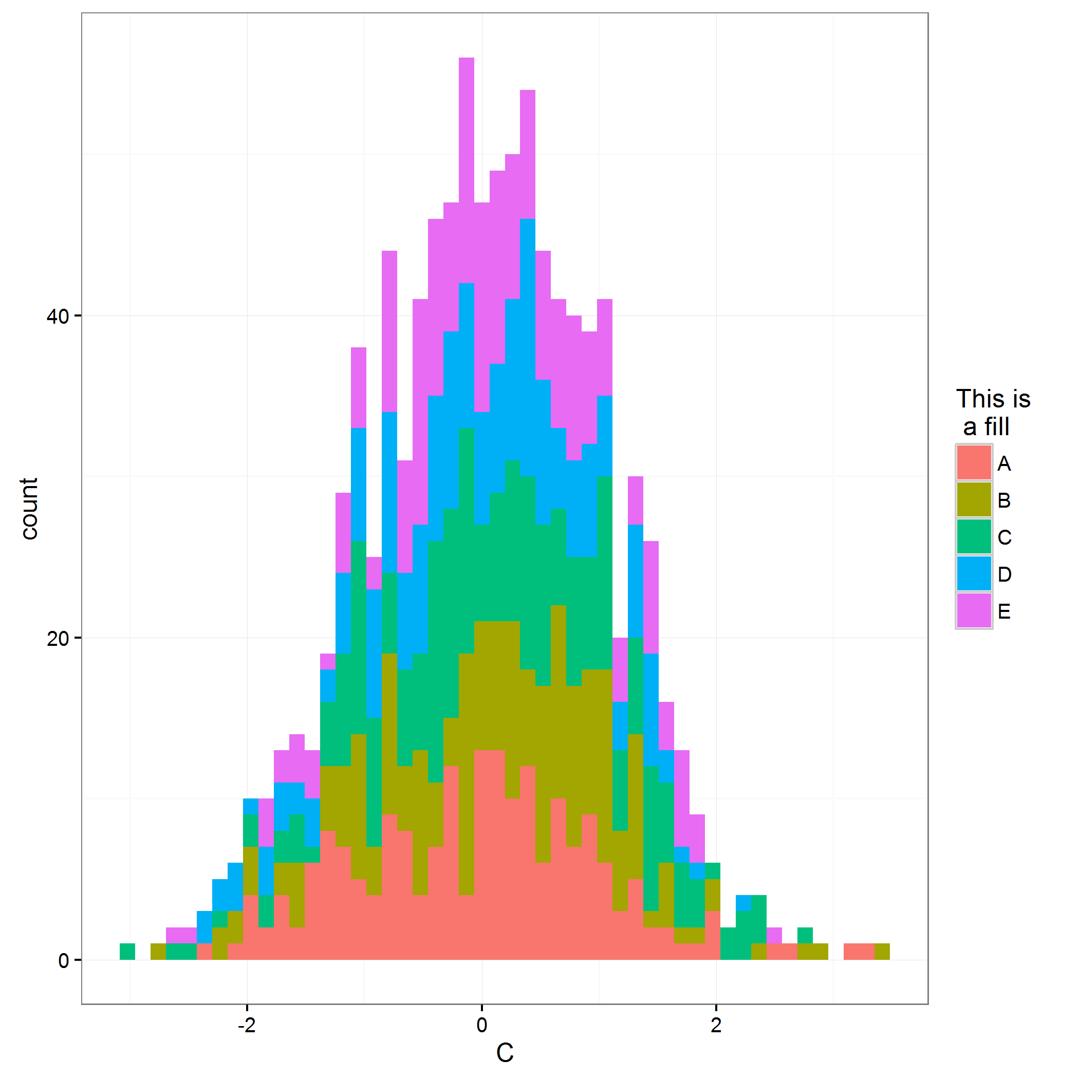

And now we will add a density, just to remember what a gaussian distribution looks like!

ggplot(data = dataset, aes(x=C,fill = B))+geom_histogram(bins = 50)+theme_bw()+
  scale_fill_discrete("This is \n a fill ")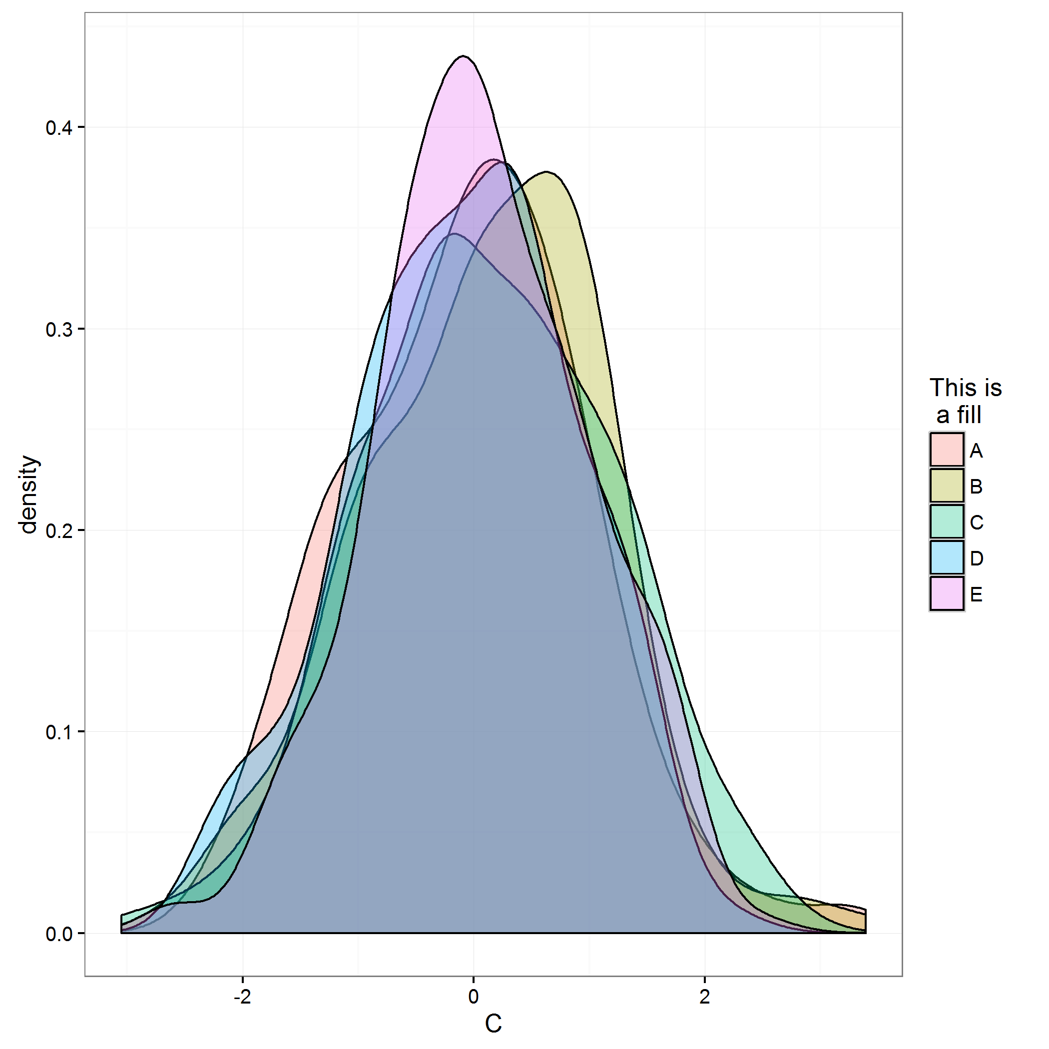

The smoothing here is a mixture of gaussians, which explains the multiple peaks, but increasing the number of observation would make all distributions converge to the same gaussian distribution: we just sampled from the same distribution at the beginning.

Saving your file

You can save your file with ggsave now:

ggsave("gaussian.png")

or

my_ggplot<-ggplot(data = dataset, aes(x=C,fill = B))+geom_histogram(bins = 50)+theme_bw()+
  scale_fill_discrete("This is \n a fill ")
ggsave(filename = "gaussian.pdf,plot = my_ggplot)

Note that ggsave automatically saves the last plot unless you specify otherwise, and will produce an image with format depending on the name of your extension (“.png”, “.pdf”,”.jpg”)

What’s next?

This closes this introduction to ggplot2. Of course there are many more things to cover, such as scales, long vs short data formatting and transitions with reshape2, heatmaps and multiple plots (with gridExtra or facet), so I’ll make more posts on these.