Machine learning exercise 1 - solution
Background
In this post I’ll solve exercise 1, with R, as I would do for a Kaggle.
I started the ML_quizz repository to help with intern selections in a machine learning team (outside of academia). Some answers are available already inside the repository, but I wanted something much more detailed and that could serve as a guide whatever your background in R/machine learning.
Data exploration
First we load the data:
dataset1<-read.table("dataset1.tsv",sep ="\t",header = TRUE)
Usually, it is a good thing to have a look at the data.
summary(dataset1)
| a | b | c | d | e | f | g | h | Y | |
|---|---|---|---|---|---|---|---|---|---|
| Min. : 1.000 | Min. :-3.54588 | Min. :-5.9946 | Min. :-8.25827 | Min. :0.0000653 | Min. : 0.000 | Min. :0.000 | Min. : 0.00 | Min. :0.0000 | |
| 1st Qu.: 3.000 | 1st Qu.:-0.70473 | 1st Qu.:-0.3366 | 1st Qu.:-1.37090 | 1st Qu.:0.2528918 | 1st Qu.: 3.000 | 1st Qu.:1.000 | 1st Qu.: 7.00 | 1st Qu.:0.0000 | |
| Median : 5.000 | Median :-0.02551 | Median : 0.9860 | Median : 0.02054 | Median :0.4945676 | Median : 5.000 | Median :1.000 | Median :11.00 | Median :1.0000 | |
| Mean : 5.509 | Mean :-0.01800 | Mean : 1.0013 | Mean :-0.01200 | Mean :0.4975494 | Mean : 5.029 | Mean :1.499 | Mean :11.67 | Mean :0.5001 | |
| 3rd Qu.: 8.000 | 3rd Qu.: 0.65778 | 3rd Qu.: 2.3738 | 3rd Qu.: 1.32180 | 3rd Qu.:0.7433941 | 3rd Qu.: 6.000 | 3rd Qu.:2.000 | 3rd Qu.:15.00 | 3rd Qu.:1.0000 | |
| Max. :10.000 | Max. : 4.32282 | Max. : 8.9656 | Max. : 6.99655 | Max. :0.9999414 | Max. :15.000 | Max. :5.000 | Max. :55.00 | Max. :1.0000 |
Here we see that all the data is numeric (no categorical variable), and that Y seem to have only two values 0 or 1. We confirm this with:
unique(dataset1$Y)
## [1] 1 0
When you have to predict a categorical variable or a state, a good place to start is logistic regression.
Sample split
To make sure that we are not overfitting the data, we need to divide the data into a training set and a testing set.
Some functions exist in caret (or scikit-learn in python) to do this. But for the sake of the explanation, I will do this manually. I will sample 70% of the dataset for training, and will test on the remaining 30%.
SplitTrain<-sample(x = 1:nrow(dataset1),size = round(nrow(dataset1)*0.7),replace = FALSE)
train<-dataset1[SplitTrain,]
test<-dataset1[-SplitTrain,]
Then I will train the logistic on the train dataset, on all columns:
logistic<-glm(formula = Y ~ ., family = "binomial",data = train)
summary(logistic)
##
## Call:
## glm(formula = Y ~ ., family = "binomial", data = train)
##
## Deviance Residuals:
##     Min       1Q   Median       3Q      Max
## -3.0726  -0.4260  -0.1146   0.4397   3.1436
##
## Coefficients:
##               Estimate Std. Error z value Pr(>|z|)
## (Intercept)  4.8079743  0.1844675  26.064   <2e-16 ***
## a           -0.0094818  0.0129360  -0.733    0.464
## b           -0.0112601  0.0372402  -0.302    0.762
## c            0.0062097  0.0190168   0.327    0.744
## d            0.0006007  0.0186309   0.032    0.974
## e           -9.8899338  0.2239260 -44.166   <2e-16 ***
## f            0.0086843  0.0167108   0.520    0.603
## g            0.0402272  0.0360426   1.116    0.264
## h            0.0030245  0.0060071   0.503    0.615
## ---
## Signif. codes:  0 '***' 0.001 '**' 0.01 '*' 0.05 '.' 0.1 ' ' 1
##
## (Dispersion parameter for binomial family taken to be 1)
##
##     Null deviance: 9704.0  on 6999  degrees of freedom
## Residual deviance: 4598.2  on 6991  degrees of freedom
## AIC: 4616.2
##
## Number of Fisher Scoring iterations: 6
We can already see that only column “e” seems to be important for our model. We can assess our model with:
prediction<-predict(logistic,test[,-ncol(test)],type="resp")
correct<- sum(as.integer(prediction >0.5) == test$Y)/length(prediction)
Notice that prediction gives the probability of Y = 1, to transform this into prediction, you have to take a threshold (here 0.5) to say if it belongs to your class or not. The fraction correct guesses in our case was 0.87%.
The glm summary warned us that some variables may not be relevant. We’ll see what happens when we train without the variables that are not relevant:
logistic2<-glm(formula = Y ~ e, family = "binomial",data = train)
summary(logistic2)
##
## Call:
## glm(formula = Y ~ e, family = "binomial", data = train)
##
## Deviance Residuals:
##     Min       1Q   Median       3Q      Max
## -3.0825  -0.4266  -0.1171   0.4394   3.1102
##
## Coefficients:
##             Estimate Std. Error z value Pr(>|z|)
## (Intercept)   4.9012     0.1169   41.92   <2e-16 ***
## e            -9.8873     0.2238  -44.18   <2e-16 ***
## ---
## Signif. codes:  0 '***' 0.001 '**' 0.01 '*' 0.05 '.' 0.1 ' ' 1
##
## (Dispersion parameter for binomial family taken to be 1)
##
##     Null deviance: 9704.0  on 6999  degrees of freedom
## Residual deviance: 4600.8  on 6998  degrees of freedom
## AIC: 4604.8
##
## Number of Fisher Scoring iterations: 6
prediction2<-predict(logistic2,test[,-ncol(test)],type="resp")
correct2<- sum(as.integer(prediction2 >0.5) == test$Y)/length(prediction2)
We now have 0.8717% correct guesses… so our model improved marginally, but we only trained on a single variable! We could also play with the threshold to improve our predictor.
To answer question 1 : only column “e” seems to play a role in the prediction.
Answer 2: Overfitting is when the model is too close to the training data (learning on the noise for example).
Answering question 3 is now pretty straightforward, construct a data frame with colomn name e, and
predict(logistic2,data.frame(e = c(0.6,0.1)),type = "resp")
##         1         2
## 0.2628562 0.9804012
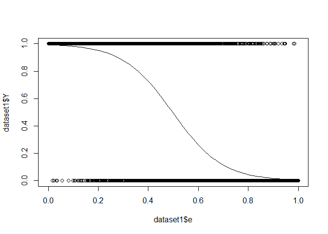
Bonus
This is what our regression looks like